I debated whether to start this blog post with either of two sentences: “R is not slow” or “R can be fast”. Starting with one of these sentences implies that I am a coward, which I am certainly not. Therefore, I am just going to come out and say it: R is not slow. Of course, it cannot compare to compiled languages such as Rust and C, but it can duke it out with the likes of Python. To prove this, I go through a variation of a function we use at work and how I made it faster with some tweaks, most of them being relatively simple.
Code
library(tidyverse)library(tinytable)create_tt <-function(data) { out <-tt(x = data) |>style_tt(i =0, bold =TRUE, color ="white", background ="blue") |>theme_html()return(out)}# The numbers quoted in the text are read from the benchmark results, so the# text always matches the tablesmedian_of <-function(b, version) { out <-as.numeric(b$median[as.character(b$expression) == version])return(out)}mem_of <-function(b, version) { out <- b$mem_alloc[as.character(b$expression) == version]return(out)}# a version's median time, to two significant figures, e.g. "900ms"about_time <-function(b, version) { out <-format(bench::as_bench_time(signif(median_of(b, version), 2)))return(out)}# how many times faster `fast` is than `slow`times_faster <-function(b, slow, fast, digits =1) { out <-round(median_of(b, slow) /median_of(b, fast), digits)return(out)}# how much faster `fast` is than `slow`, in %pct_faster <-function(b, slow, fast) { out <-round(100* (median_of(b, slow) /median_of(b, fast) -1))return(out)}# how much less memory `new` uses than `old`, in %pct_less_memory <-function(b, old, new) { ratio <-as.numeric(mem_of(b, new)) /as.numeric(mem_of(b, old)) out <-round(100* (1- ratio))return(out)}valuation_date <-ymd("2026-06-30")simulate_premiums <-function(n =10,column ="gross_premium",start =ymd("2020-01-01"),end =ymd("2026-12-31"),seed =42) {set.seed(seed) period_from <- start +sample(0:as.integer(end - start), n, replace =TRUE) above_year <-c(365:1000) above_year_prob <-0.2/length(above_year) duration <-sample(c(0, 30, 90, 182, 364, above_year),size = n,replace =TRUE,prob =c(0.02,0.10,0.18,0.20,0.3,rep(above_year_prob, length.out =length(above_year)) ) ) period_to <- period_from + duration# Premiums: right-skewed and always positive, so lognormal fits well premium <-round(rlnorm(n, meanlog =log(20000), sdlog =1), 2) out <-tibble(policy_id =seq_len(n), period_from, period_to, {{ column }} := premium ) |>mutate(total_duration =time_length(period_to - period_from, unit ="days"))return(out)}# Plots in the colours and fonts of the page. The page has a light and a dark# theme, so plot_bench() draws each plot twice and Quarto shows the one that# matches the reader's theme (`renderings` in the plot chunks)systemfonts::require_font("Alegreya", verbose =FALSE)knitr::opts_chunk$set(dev ="ragg_png")blog_colours <-list(light =c(paper ="#fffbf2",ink ="#12244d",accent ="#27548a",grid ="#c0d6df" ),dark =c(paper ="#121021",ink ="#f6f2ff",accent ="#c0d6df",grid ="#3d3870" ))# garbage collection, from none to a full (level 2) collectiongc_colours <-list(light =c(none ="#27548a",level0 ="#8e9acc",level1 ="#dda853",level2 ="#d95f0e" ),dark =c(none ="#c0d6df",level0 ="#8e9acc",level1 ="#dda853",level2 ="#d95f0e" ))theme_blog <-function(mode ="light") { colours <- blog_colours[[mode]] out <-theme_minimal(base_size =14,base_family ="Alegreya",ink = colours[["ink"]],paper = colours[["paper"]],accent = colours[["accent"]] ) +theme(plot.background =element_rect(fill = colours[["paper"]], colour =NA),panel.grid.major =element_line(colour = colours[["grid"]],linewidth =0.3 ),panel.grid.minor =element_blank(),# the expressions are code, so they get the code fontaxis.text.y =element_text(family ="Fira Code"),legend.position ="bottom" )return(out)}plot_bench <-function(data) {for (mode inc("light", "dark")) { p <-plot(data) +scale_colour_manual(values = gc_colours[[mode]],labels =c(none ="none",level0 ="level 0",level1 ="level 1",level2 ="level 2" ),name ="garbage collection" ) +# same order as the table, top to bottomscale_y_discrete(limits =rev(as.character(data$expression))) +labs(x ="time per run", y =NULL) +theme_blog(mode)print(p) }}
The Problem: Earned Premium
At work, I frequently have to calculate the earned premium of an insurance policy within a certain period. Insurance companies do not immediately recognise a premium as “earned” at the onset of a policy. They only earn this premium as the risk period decreases. In short term insurance, the policy is typically assumed to be earned uniformly across the policy period. We can summarise this in the formula:
\(EP\) is the premium earned during the valuation period
\(WP\) is the written premium of the policy
\(V_{\text{start}}\) and \(V_{\text{end}}\) are the start and end dates of the valuation period
\(P_{\text{from}}\) and \(P_{\text{to}}\) are the start and end dates of the policy
I use this across IFRS 17 reporting, reserving, experience analysis, analysing premium earning patterns etc. This is typically done every month, with datasets easily in the millions of entries, with policy duration ranging from 1 day to 20 years, depending on the class of insurance.
Version 1
At work, before IFRS 17, we used to do this in Excel. However, when IFRS 17 rolled around, Excel was just not gonna cut it anymore. Excel calculations were slow, even with the most powerful of computers, and Excel files were easily breaching half a gig of storage, with all the data transformations we needed to do before we passed data off to the IFRS 17 engine. A colleague saved us a lot of time (and uncomfortable conversations) by porting the earned premium calculations and other data transformations to R. They came up with the following function, with some improvements from yours truly:
I think this function is pretty neat. It does a couple of things:
You specify the valuation end date (column) that is then used to calculate the valuation start date, depending on the duration.
You can specify what duration you will use; one of quarterly, monthly or yearly, with a check when neither of these is selected.
You can specify what type of premium you want to do the calculations on e.g. net premium rather than gross premium.
You can specify the period from and period to columns in case you have an alternative list of dates.
I name the column at the same time as when the calculation is being done with tidy injection { }.
It handles dates natively, using a combination of base R and {lubridate}.
The functions we use e.g. pmin/pmax are all vectorised.
premiums_100k <-simulate_premiums(n =100000)# get the earliest dateearliest_date <-as.Date(min(premiums_100k$period_from, na.rm =TRUE),origin ="1899-12-30")monthly_dates <-as.character(c(seq(make_date(year =year(earliest_date),month =month(earliest_date),day =1L ),make_date(year =year(valuation_date),month =month(valuation_date),day =1L ),by ="month" ) -days(1), valuation_date))# to be used to calculate quarterly earned premiumquarterly_dates <-as.character(c(ceiling_date(seq(make_date(year = (year(earliest_date) -1), month =12, day =1),yq(quarter(valuation_date, type ="year.quarter")),by ="quarter" ),"month" ) -days(1), valuation_date))b1 <- bench::mark(v1 =map(.x = monthly_dates,.f =~calc_earned_premium(data = premiums_100k,column = .x,duration ="monthly" ) ),min_iterations =50)create_tt(data = b1[, 1:8])
expression
min
median
itr/sec
mem_alloc
gc/sec
n_itr
n_gc
v1
709ms
932ms
1.085988
2.98GB
25.15148
50
1158
Note
I am running these benchmarks on an AMD Ryzen 5 7600, a fairly powerful chip. Results may vary if you are running these benchmarks on your own.
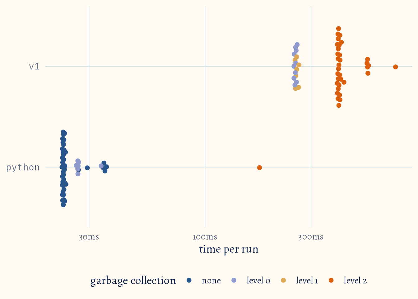
It takes about 930ms to calculate the earned premium for 100k policies, across 79 months. I was pretty satisfied with the performance of this function, with our longest running data pipeline taking about eight minutes to finish, including other data transformations, before it was passed off to the IFRS 17 engine.
I get nerd sniped
xkcd comic: Nerd Sniping
A different colleague rewrote the function in Python, and it was considerably faster than the R version, although it only takes care of the quarterly case and only accepts numerics rather than dates, and I am lazy so here:
premiums_100k_numeric <- premiums_100k |>mutate(across(where(is.Date), ~as.numeric(.x -ymd("1899-12-30"))))py_code <- r"(import calendarfrom datetime import datetimeimport numpy as npfrom dateutil.relativedelta import relativedeltadef desirialize(date): # datetime -> Excel serial number (days since 1899-12-30) return (date - datetime(1899, 12, 30)).daysdef EOMONTH(start_date, months): # Excel's EOMONTH(): move `months` months, then jump to the end of that month n_months = start_date + relativedelta(months=months) end_of_month = datetime( n_months.year, n_months.month, calendar.monthrange(n_months.year, n_months.month)[1], ) return end_of_monthdef earned_premium(df, quarter_start_date, premium, freq, pf, pt, vd): # a period ends `freq` months after it starts, or at the valuation date if EOMONTH(quarter_start_date, freq) > vd: quarter_end_date = desirialize(vd) else: quarter_end_date = desirialize(EOMONTH(quarter_start_date, freq)) # days of cover inside the period; a same-day policy counts as the one day # ending on its date, so it is earned in the quarter that contains that date policy_start = np.where(df[pf] == df[pt], df[pf] - 1, df[pf]) expired_duration = np.maximum( np.minimum(quarter_end_date, df[pt]) - np.maximum(desirialize(quarter_start_date), policy_start), 0, ) total_duration = df[pt] - df[pf] total_duration = np.where(total_duration == 0, 1, total_duration) earned_premium = expired_duration * df[premium] / total_duration return earned_premiumdef quarterly_earned_premium(raw_data, val_date, quarterly_dates): # reticulate hands over the R data frame as a pandas DataFrame (period_from # and period_to already as Excel serial numbers) and the R Date as a # datetime.date, which the functions above need as a datetime val_date = datetime.combine(val_date, datetime.min.time()) # Each quarter starts where the previous one ended, so every date in # quarterly_dates except the last one (the valuation date) is a start date. # The R versions also work out the quarter ending on the first date, so # start one quarter earlier to do the same number of quarters quarter_ends = [datetime.strptime(d, "%Y-%m-%d") for d in quarterly_dates] period_start_dates = [EOMONTH(quarter_ends[0], -3)] + quarter_ends[:-1] freq = 3 for date in period_start_dates: raw_data[date] = earned_premium( raw_data, date, "gross_premium", freq, "period_from", "period_to", val_date ) return raw_data)"reticulate::py_run_string(code = py_code)
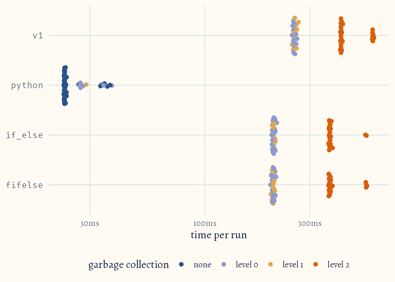
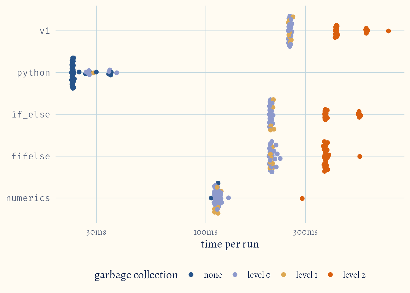
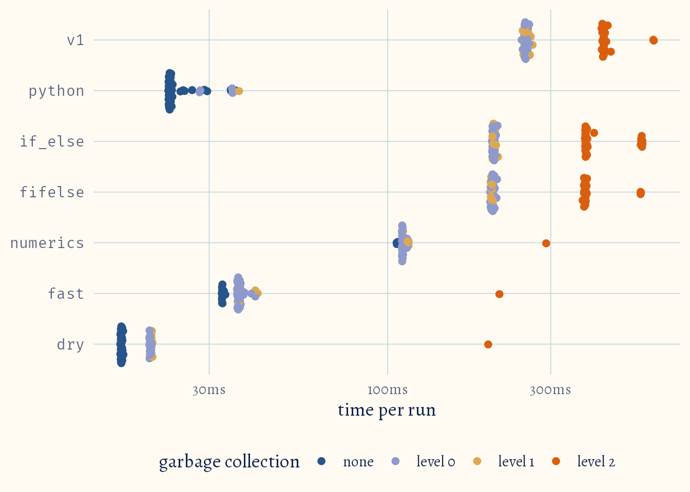
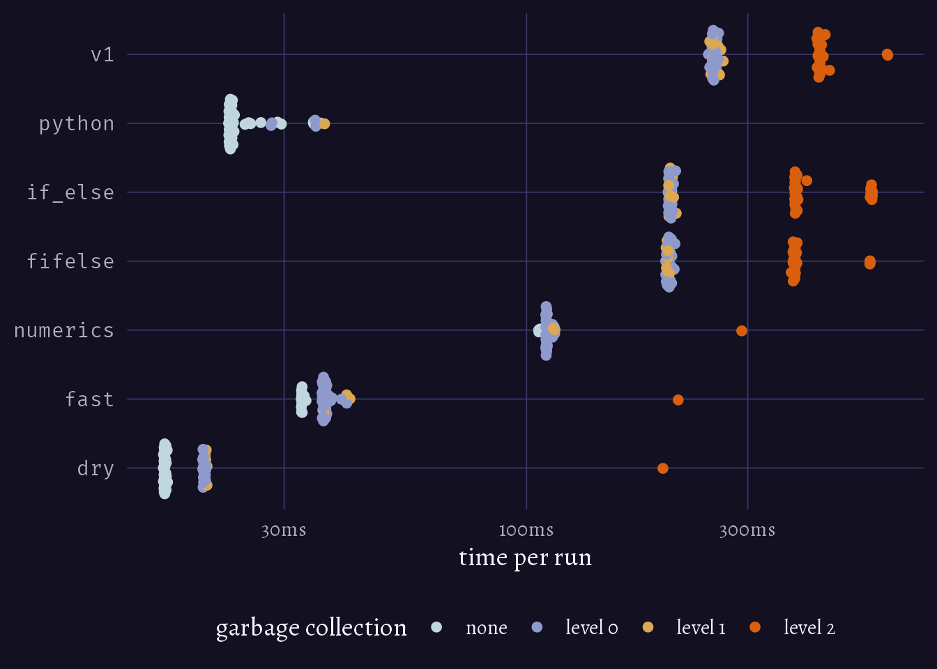
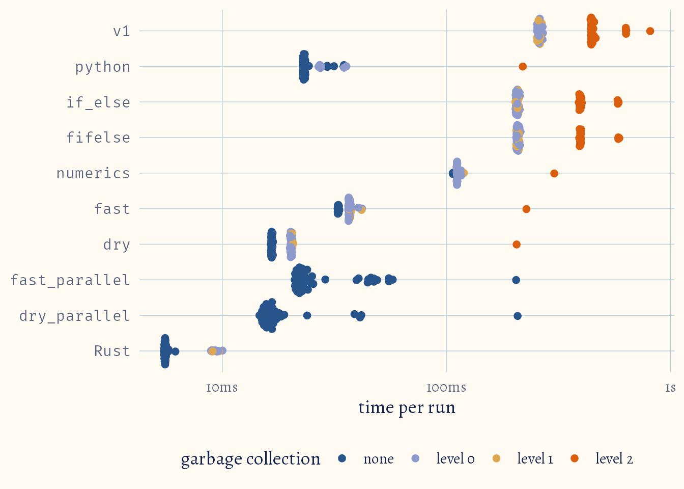
Well, this is embarrassing. Python is 17x(!!) faster than R, literally runs laps around the R version, even with the cost of passing data back and forth between R and Python.
I am a huge proponent of R. I had been preaching to my colleagues that R is not slower than Python for most use cases. After all, they are all just C and Fortran under the hood. I was crashing out when we saw these benchmarks. I absolutely needed to know why this was the case. Were my biases wrong? Sure, numpy is incredibly optimised compared to base R, but I was absolutely sure I could get the R version really close or even faster. It took me the better part of a night of work to optimise the function. One of the optimisations being incredibly obvious too. I also cheat a little.
Version 2: Use optimised functions
There exist faster versions of base R’s ifelse from popular libraries i.e. {dplyr}’s if_else and {data.table}’s fifelse, literally meaning fast ifelse. They are also safer than their base equivalent, allowing you to define what to do when NAs are introduced and also check the types of the yes/true and no/false cases. That being said, a simple replace action later:
Both functions provide speedups compared to version 1, 97% for if_else() and 99% for fifelse(), which are significant. Particularly {data.table}’s fifelse(), which by default uses half of the computer’s threads rather than one. However, this is still not quite what I am looking for.
Version 3: Types matter
Four hours in and multiple attempts later, I was getting pretty desperate. A cursory glance at the Python implementation shows a key difference with the R version. One accepts numerics, the other dates. Are date objects that much slower than numerics? Maybe? But enough to bridge the performance gap? I did not think so. It could not hurt to try though:
Why? A Date is just a number with a class attached, but that class changes which code R runs. Take pmin() and pmax(): they only use their fast C code for plain, unclassed vectors. Give them a Date and they fall back to a version written in R, which works through the vectors in several separate steps, each one going through Date’s own methods for > and [. Give them plain numbers and the whole job is done in a single pass in C, hence the speed up. This is cool and all, but the gap in performance is still pretty big.
Version 4: Just write faster code
Profiling Code
Turns out, I just write really slow code. I profiled the code using {profvis} to understand where most of the performance is going (I have to run this with a couple of dates since running this once is too fast for profvis to record anything meaningful):
ymd() is the biggest performance bottleneck of around 20ms, because it calls multiple other functions under the hood such as parse_date_time.
This is followed by tibble, yq and days at 10 ms each.
Separate from the above, pmin() and pmax() are 10ms each.
The other thing is that R absolutely loves vectors. You can get huge performance gains just from reducing everything to a vector, which we can here. With this in mind, I try to eliminate the bottlenecks, work with vectors and unintentionally find a way to get rid of the ifelse() statements:
calc_earned_fast <-function( data, column,duration ="quarterly",premium ="gross_premium",from ="period_from",to ="period_to") { rlang::arg_match(arg = duration, values =c("quarterly", "monthly", "yearly"))# convert character column to date column_date <-as.Date(column)# Replaced yq and days period_start <-as.POSIXlt(column_date) period_start$mday <-1 period_start$mon <-switch( duration,monthly = period_start$mon,quarterly = period_start$mon %/%3*3,yearly =0 ) prior_date <-as.Date(period_start) -1# Your dates are probably coming from excel so we make the adjustment here# Replaces ymd calls with a simple addition column_date <-as.numeric(column_date) +25569 prior_date <-as.numeric(prior_date) +25569# Reduce everything to a vector pf <- data[[from]] pt <- data[[to]]# reduce pf by one day when pt == pf policy_start <- pf - (pf == pt) expiry_duration <-pmax(pmin(column_date, pt) -pmax(prior_date, policy_start),0 ) total_duration <- pt - policy_start earned <- expiry_duration / total_duration * data[[premium]] out <- tibble::new_tibble(setNames(list(earned), column))return(out)}
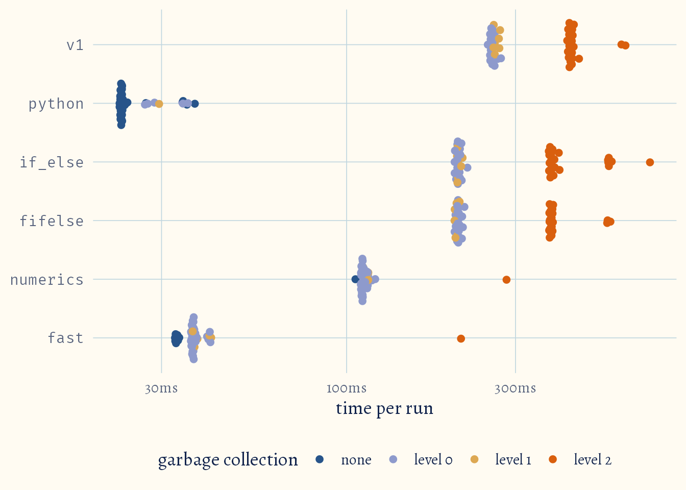
This is close. Well, closer than I have ever been. Python is still around 1.6x faster. I think I have topped out R’s performance with this specific way of computing the earned premium.
However, a cool thing about this is the reduced memory requirements for the calculations: notice the mem_alloc column in the table below. Python’s memory allocation is not accurate since bench::mark cannot measure memory outside of R:
create_tt(data =summary(b5)[, 1:8])
expression
min
median
itr/sec
mem_alloc
gc/sec
n_itr
n_gc
v1
250.5ms
421ms
2.810379
1.02GB
18.829542
50
335
python
22.8ms
23.2ms
39.861650
24.04MB
5.580631
50
7
if_else
201.9ms
216ms
3.181188
817.99MB
13.615484
50
214
fifelse
201.7ms
212.6ms
3.381715
817.99MB
12.782883
50
189
numerics
105.9ms
111.2ms
8.659434
206.34MB
11.084076
50
64
fast
32.7ms
36.9ms
24.846660
154.62MB
23.355861
50
47
The function goes from 1.02GB of memory usage to 155MB for the latest implementation. This is great. RAM is a precious resource, literally, just look at RAM prices over the last year!
Switching gears: Do not repeat yourself
A concept I find useful when speeding up code is do not repeat yourself. In other words, reduce the number of times you conduct a calculation. In this case, the policy_start and premium_per_day are calculated once, since neither changes between periods.
calc_earned_dry <-function( data, columns,duration ="quarterly",premium ="gross_premium",from ="period_from",to ="period_to") { rlang::arg_match(arg = duration, values =c("quarterly", "monthly", "yearly"))# convert character columns to dates column_dates <-as.Date(columns, origin ="1899-12-30")# only the first period needs a start date, the rest start where the one# before ended period_start <-as.POSIXlt(column_dates[[1]]) period_start$mday <-1 period_start$mon <-switch( duration,monthly = period_start$mon,quarterly = period_start$mon %/%3*3,yearly =0 ) prior_date <-as.Date(period_start) -1# Your dates are probably coming from excel so we make the adjustment here boundaries <-as.numeric(c(prior_date, column_dates)) +25569# Reduce everything to a vector pf <- data[[from]] pt <- data[[to]]# None of these change between periods, so calculate them once# reduce pf by one day when pt == pf policy_start <- pf - (pf == pt) total_duration <- pt - policy_start premium_per_day <- data[[premium]] / total_duration# Cap each boundary to the policy period i.e. no earlier than policy_start# and no later than pt capped_dates <-map(.x = boundaries,.f = \(boundary) { after_start <- dplyr::if_else( policy_start > boundary, policy_start, boundary ) out <- dplyr::if_else(after_start > pt, pt, after_start)return(out) } )# earned = days expired in the period * premium per day earned <-map2(.x = capped_dates[-1], # end of each period.y = capped_dates[-length(capped_dates)], # start of each period.f = \(.x, .y) { (.x - .y) * premium_per_day } ) out <- tibble::new_tibble(setNames(earned, columns))return(out)}
There we go, officially beat the Python version, with a slight caveat. The algorithms are not really like for like. Either way, R is not slow. Your code most likely is. We also reduce memory requirements by another 43%:
create_tt(data =summary(b6)[, 1:8])
expression
min
median
itr/sec
mem_alloc
gc/sec
n_itr
n_gc
v1
246.8ms
263.9ms
2.895070
1.02GB
15.980787
50
276
python
22.8ms
23.1ms
39.573798
24.04MB
4.748856
50
6
if_else
201.9ms
378.3ms
3.116997
817.99MB
10.473109
50
168
fifelse
199.5ms
207ms
3.403592
817.99MB
10.687279
50
157
numerics
106.2ms
110.5ms
8.726418
206.34MB
9.948116
50
57
fast
32.7ms
36.5ms
25.214698
154.5MB
21.180347
50
42
dry
16.5ms
16.7ms
46.031653
87.54MB
20.253927
50
22
Version 5: Parallelisation
I am going to cheat a little, just a little. I actually realised that this is an embarrassingly parallel problem. For the calc_earned_fast() calculation, the quarterly calculations are completely independent of each other. We can split the work across multiple workers and have them run at the same time. The same could be said for the creation of the boundaries in the calc_earned_dry() function. It’s actually pretty simple in R using {mizu} by Charlie Gao. All I have to do is set a number of “workers” with mizu_pool, replace my map with mizu_map and collect the results with mizu_collect.
cap_boundary <-function(boundary, policy_start, pt) { after_start <- dplyr::if_else( policy_start > boundary, policy_start, boundary ) out <- dplyr::if_else(after_start > pt, pt, after_start)return(out)}calc_earned_dry_parallel <-function( data, columns, pool,duration ="quarterly",premium ="gross_premium",from ="period_from",to ="period_to") { rlang::arg_match(arg = duration, values =c("quarterly", "monthly", "yearly"))# convert character columns to dates column_dates <-as.Date(columns, origin ="1899-12-30")# only the first period needs a start date, the rest start where the one# before ended period_start <-as.POSIXlt(column_dates[[1]]) period_start$mday <-1 period_start$mon <-switch( duration,monthly = period_start$mon,quarterly = period_start$mon %/%3*3,yearly =0 ) prior_date <-as.Date(period_start) -1# Your dates are probably coming from excel so we make the adjustment here boundaries <-as.numeric(c(prior_date, column_dates)) +25569# Reduce everything to a vector pf <- data[[from]] pt <- data[[to]]# None of these change between periods, so calculate them once# reduce pf by one day when pt == pf policy_start <- pf - (pf == pt) total_duration <- pt - policy_start premium_per_day <- data[[premium]] / total_duration# Cap each boundary on the workers. policy_start and pt are sent to the# workers once and shared by every boundary capped_dates <- mizu::mizu_collect( mizu::mizu_map( pool,.x = boundaries,.f = cap_boundary,policy_start = policy_start,pt = pt ) )# earned = days expired in the period * premium per day earned <-map2(.x = capped_dates[-1], # end of each period.y = capped_dates[-length(capped_dates)], # start of each period.f = \(.x, .y) { (.x - .y) * premium_per_day } ) out <- tibble::new_tibble(setNames(earned, columns))return(out)}
I am currently learning Rust and wanted to try doing this in Rust. I go for the same implementation as calc_earned_fast(). I call the Rust code using {rextendr}, with the profile set to release for faster runtime performance.
rust_code <- rextendr::rust_source(code = r"(#[extendr]fn earned_premium_rust( period_from: &[f64], period_to: &[f64], premium: &[f64], column_date: f64, prior_date: f64,) -> Vec<f64> { period_from .iter() .zip(period_to) .zip(premium) .map(|((&pf, &pt), &premium)| { // reduce pf by one day when pt == pf let policy_start = if pf == pt { pf - 1.0 } else { pf }; let expiry_duration = (column_date.min(pt) - prior_date.max(policy_start)).max(0.0); let total_duration = pt - policy_start; expiry_duration / total_duration * premium }) .collect()})",quiet =TRUE,opts = rextendr::extendr_options(profile ="release"))calc_earned_rust <-function( data, column,duration ="quarterly",premium ="gross_premium",from ="period_from",to ="period_to") { rlang::arg_match(arg = duration, values =c("quarterly", "monthly", "yearly"))# convert character column to date column_date <-as.Date(column, origin ="1899-12-30")# The prior date is the day before the period containing column_date starts period_start <-as.POSIXlt(column_date) period_start$mday <-1 period_start$mon <-switch( duration,monthly = period_start$mon,quarterly = period_start$mon %/%3*3, # January, April, July or Octoberyearly =0 ) prior_date <-as.Date(period_start) -1# Excel serial numbers, to match the data column_date <-as.numeric(column_date) +25569 prior_date <-as.numeric(prior_date) +25569# the loop over the policies runs in Rust, which reads the columns in place earned <-earned_premium_rust( data[[from]], data[[to]], data[[premium]], column_date, prior_date ) out <- tibble::new_tibble(setNames(list(earned), column))return(out)}
That is blazing fast, even with my amateur Rust code.
Julia
How about Julia? I have heard nothing but good things about Julia. It seeks to solve the “two language” problem by allowing you to write performant code in pure Julia without reaching for another language such as C or (increasingly in my case) Rust.
Note
Admittedly, I used Claude Code to write this section. I am actually pretty new to Julia, but steadily learning it. I will write my own implementation once I am comfortable with it.
julia_code <- r"(function earned_premium_julia(period_from, period_to, premium, column_date, prior_date) earned = similar(premium) for i in eachindex(period_from, period_to, premium, earned) pf, pt = period_from[i], period_to[i] # reduce pf by one day when pt == pf policy_start = pf == pt ? pf - 1 : pf expiry_duration = max(min(column_date, pt) - max(prior_date, policy_start), 0.0) total_duration = pt - policy_start earned[i] = expiry_duration / total_duration * premium[i] end return earnedend;)"JuliaCall::julia_command(julia_code)calc_earned_julia <-function( data, column,duration ="quarterly",premium ="gross_premium",from ="period_from",to ="period_to") { rlang::arg_match(arg = duration, values =c("quarterly", "monthly", "yearly"))# convert character column to date column_date <-as.Date(column, origin ="1899-12-30")# The prior date is the day before the period containing column_date starts period_start <-as.POSIXlt(column_date) period_start$mday <-1 period_start$mon <-switch( duration,monthly = period_start$mon,quarterly = period_start$mon %/%3*3, # January, April, July or Octoberyearly =0 ) prior_date <-as.Date(period_start) -1# Excel serial numbers, to match the data column_date <-as.numeric(column_date) +25569 prior_date <-as.numeric(prior_date) +25569# the loop over the policies runs in Julia earned <- JuliaCall::julia_call("earned_premium_julia", data[[from]], data[[to]], data[[premium]], column_date, prior_date ) out <- tibble::new_tibble(setNames(list(earned), column))return(out)}
Code
p <- mizu::mizu_pool(n_workers =4L)b9 <- bench::mark(v1 =map(.x = quarterly_dates,.f =~calc_earned_premium(data = premiums_100k,column = .x,duration ="quarterly" ) ),python = reticulate::py$quarterly_earned_premium( premiums_100k_numeric, valuation_date, quarterly_dates ),if_else =map(.x = quarterly_dates,.f =~calc_earned_if_else(data = premiums_100k,column = .x,duration ="quarterly" ) ),fifelse =map(.x = quarterly_dates,.f =~calc_earned_fifelse(data = premiums_100k,column = .x,duration ="quarterly" ) ),numerics =map(.x = quarterly_dates,.f =~calc_earned_numeric(data = premiums_100k_numeric,column = .x,duration ="quarterly" ) ),fast =map(.x = quarterly_dates,.f =~calc_earned_fast(data = premiums_100k_numeric,column = .x,duration ="quarterly" ) ),dry =calc_earned_dry(data = premiums_100k_numeric,columns = quarterly_dates ),fast_parallel = mizu::mizu_collect( mizu::mizu_map( p,.x = quarterly_dates,.f = calc_earned_fast,data = premiums_100k_numeric,duration ="quarterly" ) ),dry_parallel =calc_earned_dry_parallel(data = premiums_100k_numeric,columns = quarterly_dates,pool = p ),Rust =map(.x = quarterly_dates,.f =~calc_earned_rust(data = premiums_100k_numeric,column = .x,duration ="quarterly" ) ),Julia = {# copy the columns into Julia on every run, the way the Python version# copies the data frame into pandas on every run premiums_julia <-map( premiums_100k_numeric[c("period_from", "period_to", "gross_premium")], JuliaCall::JuliaObject )map(.x = quarterly_dates,.f =~calc_earned_julia(data = premiums_julia,column = .x,duration ="quarterly" ) ) },min_iterations =50,check =FALSE,relative =TRUE)mizu::mizu_pool_stop(p)create_tt(data = b9[, 1:8])
expression
min
median
itr/sec
mem_alloc
gc/sec
n_itr
n_gc
v1
45.140362
46.704555
1.000000
24898.8142
Inf
50
233
python
4.117014
4.130494
14.189000
573.3110
Inf
50
6
if_else
36.247318
69.345248
1.137673
19511.4906
Inf
50
154
fifelse
35.961292
36.585546
1.329518
19511.4906
Inf
50
144
numerics
19.226713
20.034847
3.153518
4921.7727
Inf
50
53
fast
5.896389
6.522772
9.038440
3685.4102
Inf
50
37
dry
2.955903
2.980703
16.142068
2083.9833
Inf
50
22
fast_parallel
3.803877
4.153174
10.855857
1.0000
NaN
50
0
dry_parallel
2.545380
2.784274
17.331008
555.8328
NaN
50
0
Rust
1.000000
1.000000
56.630958
491.3913
Inf
79
6
Julia
2.113030
2.305364
17.782007
493.5305
Inf
50
6
Code
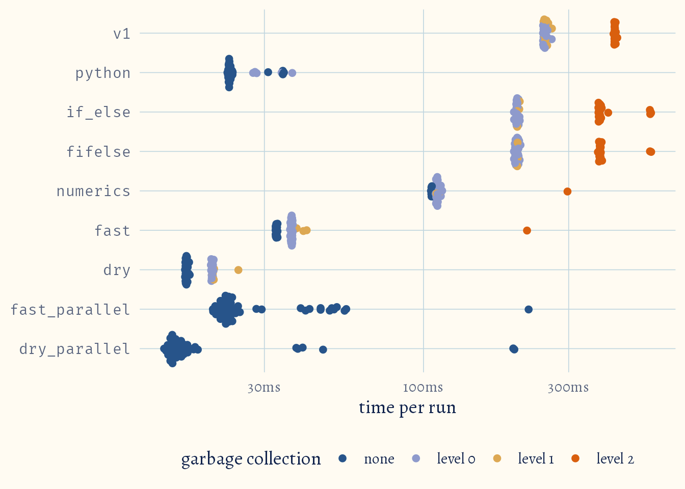
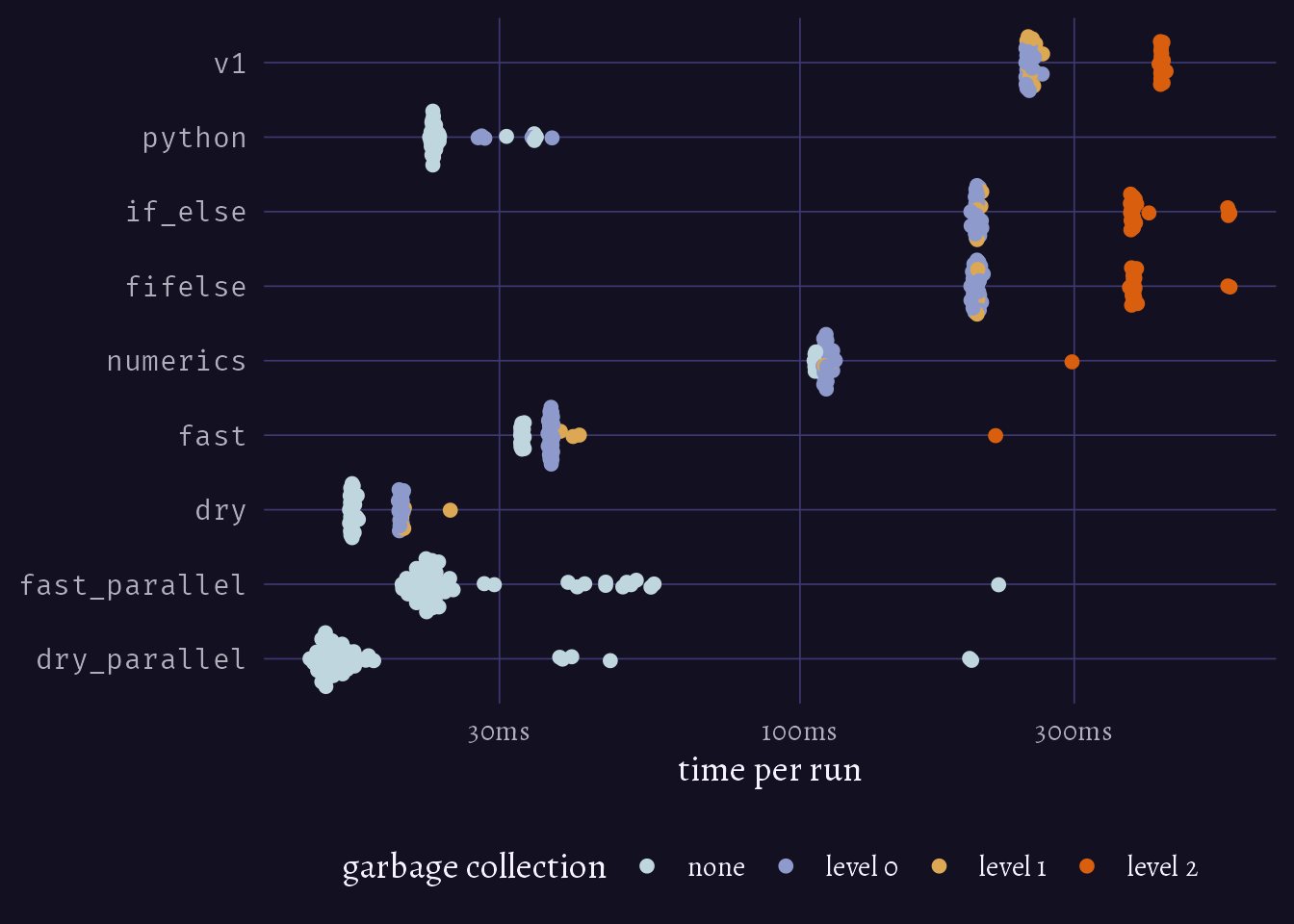
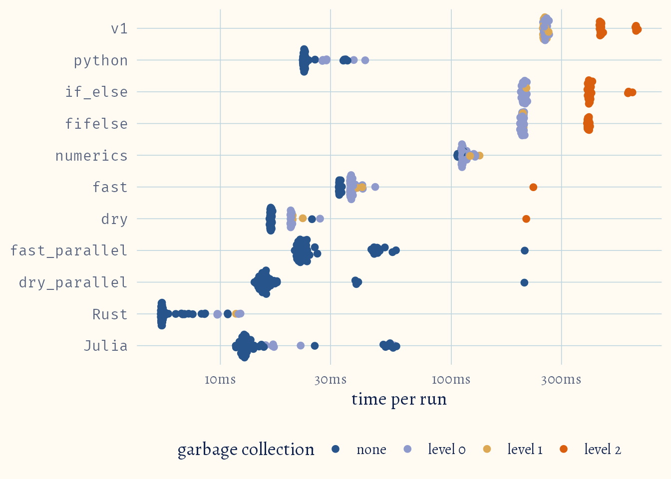
plot_bench(b9)
How well do they scale?
I have been running this on the 100k dataset. How well do they scale when there are only 10k policies? What about when I have two million policies? To be fair, I also switch the Python version to our second algorithm:
Code
py_to_date_code <- r"(import pandas as pddef quarterly_earned_to_date(raw_data, quarterly_dates): # calc_earned_dry() in Python, with desirialize() and EOMONTH() from # the Python above. Like that Python, it only does quarters # Each quarter starts where the one before it ended, so the boundaries are # the end of the quarter before the first one, then every quarter end quarter_ends = [datetime.strptime(d, "%Y-%m-%d") for d in quarterly_dates] boundaries = [EOMONTH(quarter_ends[0], -3)] + quarter_ends boundaries = [desirialize(boundary) for boundary in boundaries] pf = raw_data["period_from"].to_numpy() pt = raw_data["period_to"].to_numpy() # reduce pf by one day when pt == pf policy_start = np.where(pf == pt, pf - 1, pf) premium_per_day = raw_data["gross_premium"].to_numpy() / (pt - policy_start) # how far into its cover each policy is at each boundary: the boundary # clamped to [policy_start, pt] days_in = [np.minimum(np.maximum(b, policy_start), pt) for b in boundaries] # earned in a quarter = earned to date at its end - earned to date at its # start earned = { date: (days_in[i + 1] - days_in[i]) * premium_per_day for i, date in enumerate(quarterly_dates) } return pd.DataFrame(earned))"reticulate::py_run_string(code = py_to_date_code)
Code
# Benchmark each expression in its own fresh R session (via callr), so the# memory one version leaves behind can't change how often R collects garbage# while the next one runs. Each session gets copies of the objects its# expression uses, runs that version's `setup` (untimed) first and its# `teardown` (untimed) last, e.g. to stop a worker pool before the next# session startsbench_isolated <-function( ...,setup =list(),teardown =list(),min_iterations =50) { exprs <- rlang::exprs(...) env <-parent.frame()# Objects that code needs from the calling environments (not from packages),# including the ones used inside the functions it calls globals_of <-function(code) { todo <-unlist(lapply(code, all.names)) found <-list() packages_start <-parent.env(globalenv())while (length(todo) >0) { name <- todo[[1]] todo <- todo[-1] e <- envwhile (!name %in%names(found) &&!identical(e, packages_start) &&!identical(e, emptyenv()) ) {if (exists(name, envir = e, inherits =FALSE)) { found[[name]] <-get(name, envir = e)if (is.function(found[[name]])) { todo <-c(todo, all.names(body(found[[name]]))) } } e <-parent.env(e) } } found }# What runs inside the fresh session run_alone <-function( expr, objects, packages, setup, teardown, min_iterations ) {for (pkg inrev(packages)) {suppressPackageStartupMessages(library(pkg, character.only =TRUE)) }list2env(objects, envir =globalenv())eval(setup, globalenv())# one untimed run first, to warm up (Julia compiles on first use)eval(expr, globalenv()) out <- bench::mark(exprs =list(expr),env =globalenv(),min_iterations = min_iterations,check =FALSE )eval(teardown, globalenv()) out }environment(run_alone) <-globalenv() runs <-lapply(names(exprs), function(name) { callr::r( run_alone,args =list(expr = exprs[[name]],objects =globals_of(list( exprs[[name]], setup[[name]], teardown[[name]] )),packages =.packages(),setup = setup[[name]],teardown = teardown[[name]],min_iterations = min_iterations ) ) })# stack the runs into one bench::mark() result; its expression column can't# be stacked directly, so rebuild it with the names used here out <- vctrs::vec_rbind(!!!lapply(runs, function(run) { run$expression <-NULL run }) ) out$expression <-structure(setNames(lapply(exprs, identity), names(exprs)),class =c("bench_expr", "list"),description =names(exprs) ) out <- out[c("expression", setdiff(names(out), "expression"))]class(out) <-class(runs[[1]])# keep every run, including those with a full garbage collection. By default# bench leaves them out unless every run had one, so some sizes would be# timed with garbage collection and others without. (bench is loaded for its# summary() method)loadNamespace("bench")summary(out, filter_gc =FALSE)}
Code
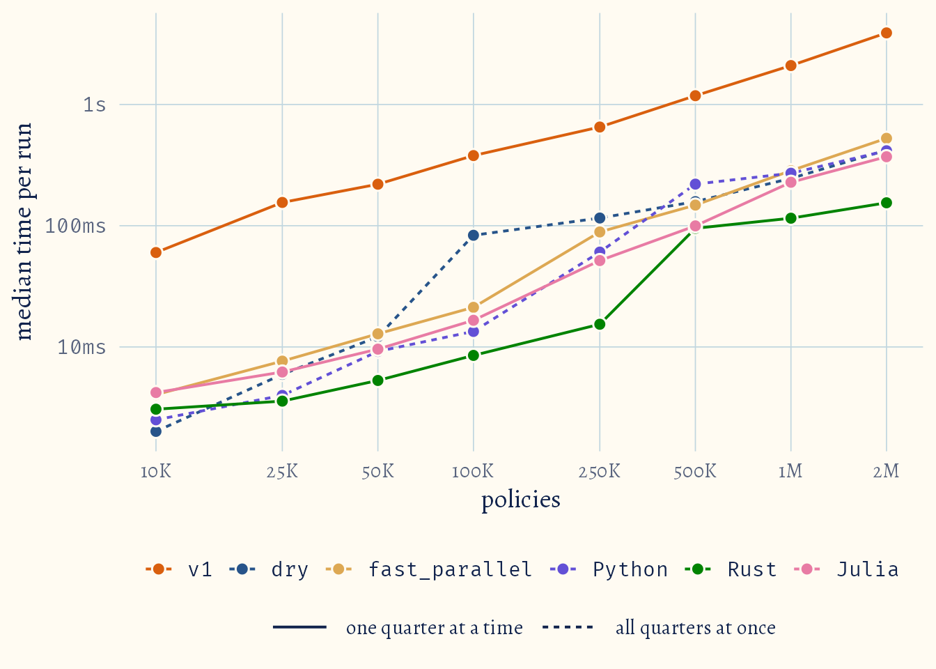
n_vals <-c(1e4, 2.5e4, 5e4, 1e5, 2.5e5, 5e5, 1e6, 2e6)# the Python that the fresh sessions should usepython_path <- reticulate::py_config()$pythonbench_scaling <-function(premiums, quarterly_dates, min_iterations =50) { premiums_numeric <- premiums |>mutate(across(where(is.Date), ~as.numeric(.x -ymd("1899-12-30")))) out <-bench_isolated(v1 =map(.x = quarterly_dates,.f =~calc_earned_premium(data = premiums,column = .x,duration ="quarterly" ) ),dry =calc_earned_dry(data = premiums_numeric,columns = quarterly_dates ),fast_parallel = mizu::mizu_collect( mizu::mizu_map( p,.x = quarterly_dates,.f = calc_earned_fast,data = premiums_numeric,duration ="quarterly" ) ),Python = reticulate::py$quarterly_earned_to_date( premiums_numeric, quarterly_dates ),Rust =map(.x = quarterly_dates,.f =~calc_earned_rust(data = premiums_numeric,column = .x,duration ="quarterly" ) ),Julia = {# copy the columns into Julia on every run, the way Python copies the# data frame into pandas on every run premiums_julia <-map( premiums_numeric[c("period_from", "period_to", "gross_premium")], JuliaCall::JuliaObject )map(.x = quarterly_dates,.f =~calc_earned_julia(data = premiums_julia,column = .x,duration ="quarterly" ) ) },# what each version needs in its fresh session, done before timingsetup =list(fast_parallel =quote(p <- mizu::mizu_pool(n_workers =4L)),Python =quote({ reticulate::use_python(python_path, required =TRUE) reticulate::py_run_string(py_code) reticulate::py_run_string(py_to_date_code) }),Rust =quote(dyn.load(rust_code[["path"]])),Julia =quote({ JuliaCall::julia_setup(verbose =FALSE) JuliaCall::julia_command(julia_code) }) ),# stop the pool, so its workers can't slow down the next sessionteardown =list(fast_parallel =quote(mizu::mizu_pool_stop(p)) ),min_iterations = min_iterations )return(out)}# Median time per version, one column per size, and how much longer the# largest size takes than the smallestscaling_table <-function(data, size, label) { ratio <-paste(label(max(data[[size]])), "vs", label(min(data[[size]]))) out <- data |>mutate(version =as.character(expression)) |>group_by(version) |>mutate(!!ratio :=sprintf("%.0fx",as.numeric(median[.data[[size]] ==max(.data[[size]])]) /as.numeric(median[.data[[size]] ==min(.data[[size]])]) ) ) |>ungroup() |>mutate(size =label(.data[[size]]), median =format(median)) |>select(version, size, median, all_of(ratio)) |>pivot_wider(names_from = size, values_from = median) |>relocate(all_of(ratio), .after =last_col()) |>create_tt()return(out)}label_policies <- scales::label_number(scale_cut = scales::cut_short_scale())scaling <- purrr::map_df( n_vals,~ { b <-bench_scaling(premiums =simulate_premiums(n = .x),quarterly_dates = quarterly_dates ) dplyr::bind_cols(n_policies = .x, b[, 1:8]) })scaling_table(data = scaling, size ="n_policies", label = label_policies)
version
10K
25K
50K
100K
250K
500K
1M
2M
2M vs 10K
v1
60.11ms
155.61ms
219.97ms
379.01ms
651.77ms
1.18s
2.1s
3.9s
65x
dry
2.01ms
5.94ms
12.15ms
83.4ms
115.73ms
158.03ms
245.75ms
420.23ms
209x
fast_parallel
4.04ms
7.64ms
12.84ms
21.22ms
88.86ms
147.95ms
284.59ms
526ms
130x
Python
2.51ms
3.98ms
9.19ms
13.43ms
60.6ms
220.35ms
270.94ms
415.28ms
166x
Rust
3.06ms
3.57ms
5.29ms
8.52ms
15.39ms
95.18ms
115.35ms
154.6ms
50x
Julia
4.21ms
6.21ms
9.59ms
16.59ms
51.59ms
99.69ms
228.23ms
370.73ms
88x
Code
# one colour per version; the order keeps colours that sit next to each other# distinguishable for colour-blind readers tooversion_colours <-list(light =c(v1 ="#d95f0e",dry ="#27548a",fast_parallel ="#dda853",Python ="#6250d6",Rust ="#008300",Julia ="#e87ba4" ),dark =c(v1 ="#d95f0e",dry ="#3987e5",fast_parallel ="#c98500",Python ="#9085e9",Rust ="#008300",Julia ="#d55181" ))# the versions that use dry's algorithm, working out every quarter at once,# are drawn dashedall_at_once <-c("dry", "Python")plot_scaling <-function(data, size, label, x_title) { points <- data |>mutate(version =factor(as.character(expression),levels =names(version_colours$light) ),algorithm =factor(if_else( version %in% all_at_once,"all quarters at once","one quarter at a time" ),levels =c("one quarter at a time", "all quarters at once") ),seconds =as.numeric(median) )for (mode inc("light", "dark")) { p <-ggplot( points,aes(x = .data[[size]],y = seconds,colour = version,linetype = algorithm,group = version ) ) +geom_line(linewidth =0.7) +geom_point(aes(fill = version),shape =21,size =2.8,stroke =0.8,colour = blog_colours[[mode]][["paper"]] ) +scale_x_log10(breaks =unique(points[[size]]), labels = label) +scale_y_log10(labels = \(x) format(bench::as_bench_time(x))) +scale_colour_manual(values = version_colours[[mode]],aesthetics =c("colour", "fill") ) +scale_linetype_manual(values =c("one quarter at a time"="solid","all quarters at once"="22" ) ) +guides(# the versions are code, so they get the code font. Their keys are# solid, so only the linetype legend shows the dashescolour =guide_legend(nrow =1,override.aes =list(linetype ="solid"),theme =theme(legend.text =element_text(family ="Fira Code")) ),fill =guide_legend(nrow =1,theme =theme(legend.text =element_text(family ="Fira Code")) ),# wider keys, so the dashes showlinetype =guide_legend(theme =theme(legend.key.width =unit(2.5, "lines")) ) ) +labs(x = x_title,y ="median time per run",colour =NULL,fill =NULL,linetype =NULL ) +theme_blog(mode) +theme(legend.box ="vertical", legend.spacing.y =unit(0, "pt"))print(p) }}plot_scaling(data = scaling,size ="n_policies",label = label_policies,x_title ="policies")
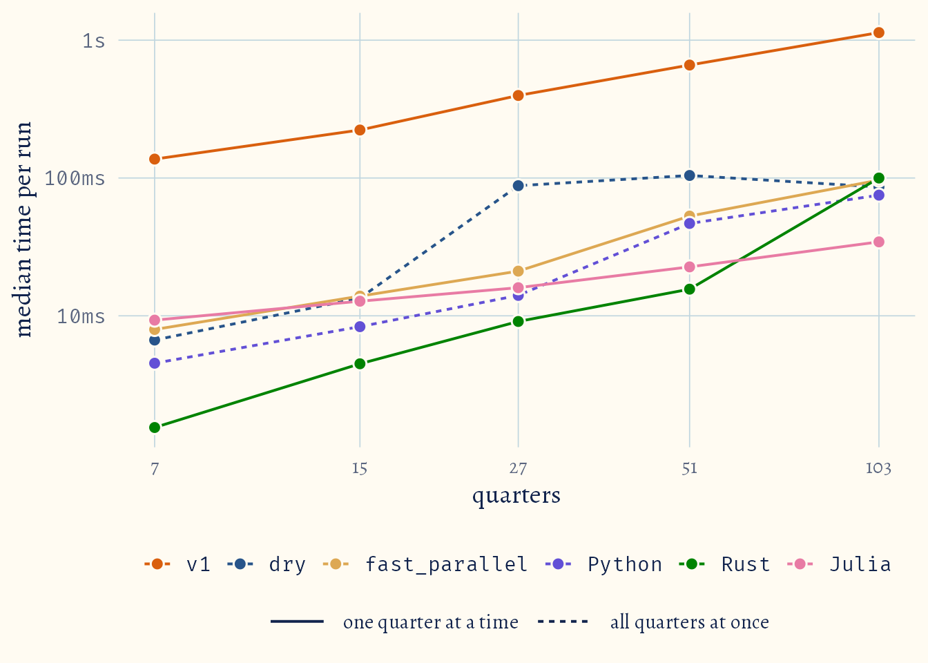
What about more quarters? Here I keep 100k policies, but move their start dates further back, so there are more quarters to calculate:
Code
# the quarter ends from the quarter before the earliest policy starts up to# the valuation date, worked out the same way as quarterly_datesquarter_ends <-function(data) { earliest_date <-min(data$period_from, na.rm =TRUE) out <-as.character(c(ceiling_date(seq(make_date(year = (year(earliest_date) -1), month =12, day =1),yq(quarter(valuation_date, type ="year.quarter")),by ="quarter" ),"month" ) -days(1), valuation_date ))return(out)}start_years <-c(2025, 2023, 2020, 2014, 2001)scaling_quarters <- purrr::map_df( start_years,~ {# policies start between 1 January of that year and the end of 2026 premiums <-simulate_premiums(n =1e5,start =make_date(year = .x, month =1L, day =1L) ) dates <-quarter_ends(data = premiums) b <-bench_scaling(premiums = premiums, quarterly_dates = dates) dplyr::bind_cols(n_quarters =length(dates), b[, 1:8]) })scaling_table(data = scaling_quarters,size ="n_quarters",label = \(x) paste(x, "quarters"))
The biggest speed ups I got were from rewriting how to do the calculations. For example, calc_earned_dry() was faster than the original Python code due to a superior algorithm. Most bottlenecks in code written for basic actuarial work come down to how well the code was written.
Python just beat out R, even in the dry versions, but just barely. Besides, what are you going to do with a couple of milliseconds? I do have to give numpy and its optimisations credit.
Parallelisation is not always going to be faster. For this particular use case, the function is already fast, without parallelisation. By the time it takes to set up the workers and copy the data into shared memory, non-parallelised code would already be close to finished. I do have some ideas where the benefits for it would be much greater so stay tuned for those posts.
For truly performant code, just reach for Julia or Rust. Julia does start out slow because of the compiler starting up, but quickly caught up with Rust. Rust is just blazing fast, either way.
It’s pretty cool that I can call all these languages from R, in the same session too. It is pretty easy for a polyglot to pick the right tool for the job depending on what bit of analysis you are doing. Anyways, I had fun. Think you can beat these implementations? Let me know, shoot me an email at gicherumichael@fastmail.com. I will be sure to update this post as more implementations come in.